Materials Informatics Book

Should I write a technical "how-to" textbook?

Why am I asking this question, well, I've come to somewhat of a cross roads in materials informatics. I have digested a lot of research papers and review monographs [1-4], but constantly run into the following problem:

How do I implement the technique discussed, reproduce the results, and extend it towards my specific domain topic?

The answer over and over is, these resources aren't going to enable that or provide a way to do so. Yes in some cases there are Github repos that provide the source, but what I find is the data input pipeline is so complicated or convoluted that figure out how to get my data to work is too much effort. It would just be better to actually implement the model from scratch based on my specific data preprocessing/pipeline.

So why would me writing a address this challenge? Well, for one no one else has written such a book. You have three textbooks available on this topic:

• Isayev, O., Tropsha, A., & Curtarolo, S. (2019). Materials informatics: Methods, tools, and applications. John Wiley & Sons. url.
• Rajan, K. (2013). Informatics for materials science and engineering: Data-driven discovery for accelerated experimentation and application. Butterworth-Heinemann. url.
• Kalidindi, S. R. (2015). Hierarchical materials informatics: Novel analytics for materials data. Elsevier. url.

There are a few other monographs [3-4] that try to focus on specific subdomain areas of materials science. The books above are actually pretty good if your looking for a foundational understanding of data science and machine learning applied to materials science and engineering. The problem with those books is they are more reference text for people involved in materials informatics. They won't help you get going in front of a computer or information systems.

This is what is missing and I want to provide a solution. One reason is that I'll learn more by writing a book. The second reason is I think the tools are now available to make writing this type of book much smoother. Writing literate programming is a regular thing (e.g., Jupyter notebooks) and therefore writing while coding is straightforward, usually.

The dilemmas I face are what programming language to use, what framework to write in, how much to cover, and best examples/case studies to use. For the programming language its between Python and Julia. I'm torn because I prefer to use Julia but Python is more broadly adapted and has very mature and standard packages (e.g. scikit-learn, pytorch). For the framework its also a challenge. I'm favoring Quarto at the moment and it won't matter if I use Julia or Python. Similar case for Jupyter Books. I haven't used Jupyter Books and I'm not too interested in adapting the MyST. There are other options to explore as well, such as Books.jl which is geared towards PDF and website generation.

For the content the book would cover, I need to be very thoughtful. My rough outline would be something like:

1. What is data and information
2. Describing data: Probability, Statistics, and Visualization
3. Processing & Transformation of data
4. Pattern extraction and reduced representation
5. Regression, optimization, and prediction
6. Neural network models
7. Autonomous solution seeking

The first 3 chapters are probably self-explanatory, the chapters 4,5, and 7 would correspond to unsupervised, supervised, and reinforcement learning. This is a moving target so it would change based on my particular interest and focus.

The key point is that each chapter provides the background and the code to actually do something at the computer. My goal would also be to try to do as much as possible from scratch. Meaning, that if it made sense I would actually have a section in the chapter on neural networks that builds the layers, does forward and backward propagation, and trains using minimal packages (e.g. NumPy). Why do so if in the end we all are going to implement and deploy using pytorch or `tensorflow? Because for most the act of doing is what solidifies understanding and comprehension. After coding up a simple NN, when someone talks about backpropagation, you'll know what is actually being down, at least from the most minimal implementation ¹.

Status

I have yet to really start writing, but plan to have some kind of a draft by end of 2024. My goal would be to make the draft available online first. For the physical copy I intend to go the self-publishing route using Amazon Kindle services.

As for the applications and case studies used, well, I really want these to be real in the sense that they have either been done in academia or industry. I want to try and avoid "toy problems" not because they aren't useful but because I want to avoid the issue with a creating a insurmountable barrier to applying whats in the book the readers specific interest/problem.

My hope for this potential book is that grad. students and researchers who want to get into this area, but don't have any hands-on experience, can more easily do so by working through the book. The book obviously wouldn't be at the forefront of research methods, but it would be as if you were taking a graduate level lab at a major university.

References

[1] K. Takahashi and L. Takahashi, "Toward the Golden Age of Materials Informatics: Perspective and Opportunities", J. Phys. Chem. Lett., vol. 14, no. 20, pp. 4726-4733, May 2023, doi: https://doi.org/10.1021/acs.jpclett.3c00648.

[2] C. Li and K. Zheng, "Methods, progresses, and opportunities of materials informatics", InfoMat, p. e12425, Jun. 2023, doi: https://doi.org/10.1002/inf2.12425.

[3] T. Lookman, F. J. Alexander, and K. Rajan, Information science for materials discovery and design. Springer, 2015.

[4] I. Tanaka, Nanoinformatics. Springer, 2018.

Footnotes

---

1. There are different numerical implementations to achieve backpropagation and the book I would write showing how to implement a NN would focus on the most basic approach. ↩

Reuse and Attribution

Notes: Equivariant Features

By chance, I came across a presentation [1] by Professor Tess Smidt at MIT on equivariant neural networks; its really concise and clear introduction and I highly recommend it. I took some notes during the presentation, which I'm logging here, but practically the same content is available in her slides which can be found here. Her group also maintains a package called e3nn [2]. Below are my notes, which I'll probably revisit to update and turn into a more formal blog.

Notes

• Invariant neural networks (NN) means the outputs will be the same regardless of the transformations performed on the inputs, i.e., scalar representation.
• Equivariant NN means the transformations applied are global and get pass through to the outputs but consistently. In other words if we apply a transformation on the inputs the same transformation gets applied on the output. You can think of this as vector outputs that can be rotated.
• In higher order equivariant representations you can have very data efficient learning.
• Physical systems use coordinate systems (i.e. Euclidean geometry) to describe the physical system, we get to choose!
• Transformations between coordinate systems in Euclidean space utilize proper symmetries.
• I spoke a bit about this in my post on Graph NN potentials.
• Equivariant NN will understand the same motifs even if they are rotated or in different locations.
• How do you build a equivariant NN
• Irreducible representations to express transformations, i.e., symmetry groups.
• Spherical harmonics to featurize the geometry --> that is what are the basis functions that give use a geometry
• Tensor products to build a representation. (equivariant multiplication)

Example

Take simple, moving, two-particle system representation and indicate how it transforms.

• Define the coordinate system geometry geometry = [[x0, y0, z0], [x1, y1, z2]]
• Specify the features, which are present features = [[m0, v0x, v0y, v0z, a0x, a0y, a0z], [m1, v1x, v1y, v1z, a1x, a1y, a1z]]
• Construct the irreducible representation group, i.e. $\mathit{O}(3)$
• Using the e3nn package define the scalar and vector symmetries: scalar = e3nn.o3.Irrep('0e') , vector = e3nn.o3.Irrep('1o')
• Here the parity is encoded in the e or o , i.e., flip sign under inversion/mirroring.

Irreducible representations

• So we want to define the fundamental transformations that exist for objects/features.
• Higher-dimensions features, the data is represented as tensors in 3D space.
• The transformations of these data types is done using hydrogenic atomic spherical harmonics of differnt angular momentum.
• For example a scalar is transformed by L=0 or s-orbital, where as a vector is transformed through L=1 or p-orbital. Furthermore, a matrix would be transformed through L=2 or d-orbital.

Basis of descriptors: Spherical Harmonics

• Given a distance vector of one atom to another atom, $\vec{r}_{ij}$, find the spherical projections, i.e., convolution, we have $\sum_{lm} Y_{lm}(\hat{r}_{ij})Y_{lm}(\hat{x})$
• This gives a magnitude and a sign of the coefficients. Can think of it as an array of these. In addition, it is possible to map these coefficients on to a sphere where the radius from the center of the sphere is the magnitude.
• Now if you have $N$ atoms you can calculate these coefficients for every pairing with $i$ we can take linear sum given these harmonics form a orthogonal basis (i.e. vector space)
• This gives a nice fixed signal length and describes a distribution of vectors.
• The linear sum cancels out many components because many of them are just rotations of the same signal and therefore symmetry of the environment cancels out certain irreducible representation
• Fairly robust against noise in the signal.

Tensor Products

• So how do we create more complex features/descriptors: multiply them.
• This is similar to a kernel method but here we use tensor products, ex., $(x,y,z)\otimes(x,y,z) = (x^2,xy,xz,y^2,yz,z^2)$.
• Rotations acting on such features space are dense (reducible) but we can decompose the rotations into a irreducible representation by changing basis, where the space now is more block diagonal.

Creating equivariant signals

• Combining the spherical harmonic projections with tensor products provides invariant signals.
• Recall spherical harmonic projections are equivariant because rotation of the coordinate system changes the function.
• Power spectra, $x ⊗ x$, Bispectra, $x ⊗ x ⊗ x$, etc.
• Bicspectra will consist of scalars and pseudoscalars and smooth under distortion and break symmetry.

Applications: Clustering local environments of materials

• Can find the different symmetries in local environments by determining the Bispectra terms, i.e., can use higher order representation to enable expressive features of local atomic environments.
• Check out https://e3nn.org.

References

[1] Smidt, T., Harnessing the properties of equivariant neural networks to understand and design materials, From Molecules to Materials: ICLR 2023 Workshop on Machine learning for materials (ML4Materials), May, (2023). https://iclr.cc/virtual/2023/14141.

[2] Geiger, M., and T. Smidt. E3nn: Euclidean Neural Networks. arXiv, (2022). https://doi.org/10.48550/arXiv.2207.09453.

Reuse and Attribution

Automating dataset labeling

Could you use a LLM to label a material simply by using the crystal structure expressed in natural language?

I'm trying to see if this is true or not with the recent explosion of tools. I came across the tool Autolabel which uses LLMs to automatically label datasets with human level accuracy but using a fraction of the time. As to the technical details, its not clear what the clear advantage of this library other than it make use of few shot prompt engineering and similarity search to get the best LLM accuracy to label data.

So how do I think I might use this? Well What if you could label a material as magnetic or non-magnetic simply from a description of the crystal structure. How do you describe a crystal without using standard crystallography notation. Well in truth, the cif format is just formatted text, so you could use that, but the standard is very broad and the format can contain sparse details. What we can do is use a tool called Robocrystallographer which will describe a crystal structure from a format file such as cif or POSCAR and describe the environment in significant detail. This type of description is ideal for something like labeling.

The question now is if the information is expressive enough for a LLM to understand the context for what makes something magnetic or non-magnetic. So here is an example of a few shot prompt setup:

You are an expert in magnetic crystalline materials. Your job is to classify the magnetic ordering of a crystal into one of the following labels:
Non-magnetic
Magnetic

You will return the answer with just one element: "the correct label"

Some examples with their output answers are provided below:

Input: Cs(MoS)₃ crystallizes in the hexagonal P6₃/m space group. Cs is bonded in a 9-coordinate geometry to nine equivalent S atoms. There are three shorter (3.60 Å) and six longer (3.73 Å) Cs–S bond lengths. Mo is bonded in a distorted see-saw-like geometry to four equivalent S atoms. There are a spread of Mo–S bond distances ranging from 2.49–2.60 Å. S is bonded in a 7-coordinate geometry to three equivalent Cs and four equivalent Mo atoms.
Output: Non-magnetic

Input: CuCr₂Se₄ is Spinel structured and crystallizes in the cubic Fd̅3m space group. Cr³⁺ is bonded to six equivalent Se²⁻ atoms to form CrSe₆ octahedra that share corners with six equivalent CuSe₄ tetrahedra and edges with six equivalent CrSe₆ octahedra. All Cr–Se bond lengths are 2.52 Å. Cu²⁺ is bonded to four equivalent Se²⁻ atoms to form CuSe₄ tetrahedra that share corners with twelve equivalent CrSe₆ octahedra. The corner-sharing octahedral tilt angles are 57°. All Cu–Se bond lengths are 2.37 Å. Se²⁻ is bonded in a distorted rectangular see-saw-like geometry to three equivalent Cr³⁺ and one Cu²⁺ atom.
Output: Magnetic

Now I want you to label the following example:
Input: SrSn(PO₄)₂ crystallizes in the monoclinic C2/c space group. Sr²⁺ is bonded in a 8-coordinate geometry to eight O²⁻ atoms. There are a spread of Sr–O bond distances ranging from 2.61–2.99 Å. Sn⁴⁺ is bonded to six O²⁻ atoms to form SnO₆ octahedra that share corners with six equivalent PO₄ tetrahedra. There are a spread of Sn–O bond distances ranging from 2.03–2.10 Å. P⁵⁺ is bonded to four O²⁻ atoms to form PO₄ tetrahedra that share corners with three equivalent SnO₆ octahedra. The corner-sharing octahedral tilt angles range from 41–50°. There are a spread of P–O bond distances ranging from 1.52–1.58 Å. There are four inequivalent O²⁻ sites. In the first O²⁻ site, O²⁻ is bonded in a distorted bent 150 degrees geometry to one Sn⁴⁺ and one P⁵⁺ atom. In the second O²⁻ site, O²⁻ is bonded in a distorted single-bond geometry to two equivalent Sr²⁺ and one P⁵⁺ atom. In the third O²⁻ site, O²⁻ is bonded in a 3-coordinate geometry to one Sr²⁺, one Sn⁴⁺, and one P⁵⁺ atom. In the fourth O²⁻ site, O²⁻ is bonded in a 3-coordinate geometry to one Sr²⁺, one Sn⁴⁺, and one P⁵⁺ atom.
Output:

Now if I use Autolabel I can test out how this might work for different OpenAI models or even other LLMs. In addition, details on the level of confidence (not sure how this is calculated) are provided on the labels. The threshold for a good confidence level of a label is also provided based on my understanding. So say you have a label with 30% confidence that it is correct, but the threshold is around 55% for a reasonable confidence then this label would be rejected.

First results

So I went ahead and tried this out and if I can get it to work, I'll probably try to write a preprint. However, my early attempts are proving that this isn't much better than a random guess, or in some cases even worse. I actually did this on the magnetic ordering labels rather than on magnetic vs. non-magnetic, here are some example data points:

Although the confidence level is high for all labels, the accuracy is abysmal, 17%. This is why the threshold value seems to be needed as a guide for accepting labels, in this case the threshold needs to be increased. I have seen that for more prompt shot examples it gets a bit better. The use of GPT-4 also seems to improve the accuracy considerably but the cost is very high. It probably would have been better just to use the labels magnetic and non-magnetic since magnetic ordering has its own symmtry related to electron spin which won't be captured by the description generated from Robocrystallographer.

As I do more on this I'll share my code but at the moment I'm holding off since it needs some further testing. Also I'm hoping to publish this on my spare time if it shows significant promise in being able to label crystal structures from natural language descriptions. You can imagine other labels like whether or not a material is piezoelectric.

For me to be convinced this is the way to go, the accuracy on a test dataset needs to be in the 90% range. This is just an opinion and my bias towards wanting high-quality labeled data to then go do other stuff with the labeled dataset. I'll probably write an update to this post as I keep playing around with this.

Update, 26 June, 2023

I've been trying this approach out and have been able to get better performance, especially when using GPT-4. The problem is the cost for labeling a dataset with 1000 entries is high. I've been able to get the accuracy higher, close to 70%, but the problem is in practice I would only want to keep labels with confidence scores > 90% and many of the labels have very low confidence scores and therefore are probably just good guesses by the LLM.

References

1. [1] Autolabel. https://github.com/refuel-ai/autolabel. Accessed 21 June 2023.
2. [2] Ganose, Alex M., and Anubhav Jain. “Robocrystallographer: Automated Crystal Structure Text Descriptions and Analysis.” MRS Communications, vol. 9, no. 3, Sept. 2019, pp. 874–81. Springer Link, https://doi.org/10.1557/mrc.2019.94.

Reuse and Attribution

Useful Linux Command Line AI Tool

I've been looking for a Linux command line tool that leverages AI to streamline my terminal experience. There are so many instances where I forget a command or what to do some convoluted sequence of shell commands where it takes me a whole lot of time to figure it out. This is way easier now with LLMs but moving back and forth between the terminal and browser isn't the smoothest and the browser doesn't have access to my local device. Although letting an AI system run this on your local device is pretty scary when you think about it, I mean imagine if you give it a prompt and it incorrectly interprets the meaning and ends up deleting important files and the backup you may have for those files. For this reason, make sure you have cloud or isolated/disconnected backups.

Initially, I came across Warp, which seems extremely powerful and has mostly what I want, however, there is no current Linux version. Then I found Fig.io but couldn't get this to configure properly and it seems the AI tool is only special access. So I kept searching and eventually found Yai. The thing I like about yai is it was easy to install/configure,  

curl -sS https://raw.githubusercontent.com/ekkinox/yai/main/install.sh | bash

This command will install Yai for you. Then to initialize and use just type:

user@system:~$ yai

 

in your terminal and it will prompt you for your OpenAI key. If you want to specify any types of details related to OpenAI model or pre-prompt context, you can modify the file below,

user@system:~$ emacs .config/yai.json

Once everything is configured it's pretty cool what you can do. There are two options, the first is to run yai in execute mode with the flag -e which will generate shell commands and any other text/code based on the prompt you give it. You are then prompted to whether you want to run the command, you should review what yai shows to make sure you don't do any harmful operations. The other mode is -c which is used yai in a chat-based mode. This is good for general inquiries. At the moment yai doesn't have internet access itself and is limited by the OpenAI model token context size. This means you can't just pipe to it any arbitrary sized document or code to help you understand it. To get around this you can use commands like head.

It would be nice if yai used vector stores and other tools (e.g. similar to Langchain) to enable questions and answering of your documents and code. I would take a stab at it but the problem is yai is written in the Go programming language which I have absolutely no experience with. The tool is still very useful though as I'll show below.

A somewhat complicated example

First, let me give some context about what I'm doing with this example. I want to ask yai to create a LAMMPS simulation script and then use the Linux task spooler utility to schedule the simulation job. So here is the prompt I gave it (after a few iterations, a little on that later) was:

yai -e " I want you to create a folder in my home directory called simple_job; if the folder exist just delete it. In the folder please create a LAMMPS molecular dynamics script using the lennard-jones potential for Argon gas in a box with lengths 20 angstroms (ex. region 1 block 0 20 0 20 0 20), be sure to create 100 randomly placed Argon atoms in the box  and set mass. You can use a NVT ensemble and set the temperature to 300 Kelvin and run the simulation for 1000 timesteps. Make sure you validate all the LAMMPS commands you use. After creating the LAMMPS script, I want you to use the task-spooler, command 'tsp', to run the command to run is 'mpirun -np 1 /opt/lammps/23Jun2022/build/lmp -sf omp -in {NAME_OF_SCRIPT}' where {NAME_OF_SCRIPT} is the name you used for the LAMMPS simulation script you created in the folder simple_job."

So what did this give in terms of the commands? At first it looks a bit difficult to go through and what you see is that it strings all the commands together and for the script it uses echo. Here is the output:

`mkdir -p ~/simple_job && rm -rf ~/simple_job && mkdir -p ~/simple_job && cd ~/simple_job && echo -e 'units lj      
  atom_style atomic                                                                                                   
                                                                                                                      
  lattice fcc 0.8442 region simbox block 0 20 0 20 0 20 create_box 1 simbox create_atoms 1 random 100 12345 simbox    
  mass 1 39.948 pair_style lj/cut 2.5 pair_coeff 1 1 1.0 1.0 2.5 velocity all create 300.0 12345 fix 1 all nvt temp   
  300.0 300.0 0.1 thermo 100 thermo_style custom step pe temp press run 1000' > simulation.lammps && tsp mpirun -np 1 
  /opt/lammps/23Jun2022/build/lmp -sf omp -in simulation.lammps`                                                      

  Create the folder simple_job, delete it if exists, and create the LAMMPS script with the desired parameters. Then use 

  confirm execution? [y/N]

Is this correct, does it work? The LAMMPS commands don't look like they are on newlines but indeed they are when you look at the final file produced. Did it run, it did! It submitted the task to tsp and the LAMMPS script actually ran. This is pretty cool if you ask me, especially if you want to create a draft template simulation folder/file setup.  Below is the simulation result visualized which seems to run without any wonky behavior even though the pair potential coefficients are not correct. I had to manually add the dump command but I could have specified this in the prompt.

Simulation result from a prompt given to Yai.

Caveats

The example above didn't work smoothly on the first try, well yai did always carry out all the steps, however, the LAMMPS script regularly contained errors. This is do to the GPT models' limited knowledge of LAMMPS so it's not an issue with yai. This is where some kind of vector store or other tools to help yai know about the details of the commands it's going to use or code/script it will produce. If I could have told yai, "Be sure to review the LAMMPS documentation so that you use the correct syntax, commands, and arguments" this probably would have helped. I think it took me about 5 iterations to get the prompt to work. The changes I usually had to make were related to the details of the LAMMPS script.

Where to go from here

You can see that these types of tools are going to change how computational work is done. Its going to improve efficiency and ease of use for complex sequences of steps that are typically done when computing. My hope is that these tools only get better and can incorporate documents or other resources as part of the generative output.

Reuse and Attribution

Interest in Materials

Note

I've been informed that occassionally trends.google.com refuses connection and thus the embedded graphs aren't being displayed. Not sure what the best option is here other than static versions, however, if its not showing for you I would just go to trends.google.com and manually use the terms, Materials Science, Materials Engineering, etc.

I was curious whether or not there has been an increase in the number of people interested in materials science and engineering. My initial hypothesis was "I have a strong belief that people are more interested given that most advances in technology will require new materials". With that said I started to look at Google trends to see if I could use any data they collect and sure enough they let you look at search trends. So what is the search trend over the last 20 years for materials science and engineering? Below are the results:

Turn's out my hypothesis, based on Google trends data, is not true. More specifically, it seems the keywords I used with google trends aren't trending up. You actually see a trend down or constant. We can also look at how the interest is distributed across different countries.

I'm a bit curious why it was higher in 2004-2005 and then dropped off and has been constant since then.

Reuse and Attribution

Refresher: Bessel Functions

 Let's talk about Bessel functions! First, who was Bessel? Friedrich Bessel was a German astronomer and mathematician whose namesake was given to the solutions used to solve a specific type of differential equation. The differential equation in question is the following:

\begin{equation}x^2\frac{d^2y}{dx^2} + x\frac{dy}{dx} + (x^2-n^2)y = 0\label{eq:ode}\end{equation}

This is a second-order linear ordinary differential equation and is known as a canonical ODE because its solutions are special types of functions. For those unfamiliar with second-order linear ODEs let me explain ( I often forget so it's helpful for me as well). The "second-order" just means the highest derivative in the equation, in this case, its two. The ordinary is because there is only a single independent variable $x$. Linear indicates that we don't have terms like $y^2\frac{dy}{dx}$, in other words,  the dependent variable and its derivatives only appear to the first power and the coefficients are not in terms of the dependent variable. There is also the case that this equation is homogenous because $y$ is involved with every term.

The solutions to the Bessel equation are called Bessel functions. The functions form a basis because they are linearly independent and there are two flavors of functions called the "first-kind" and the "second-kind". The first-kind, usually denoted as $J_n(x)$, has the form:

\begin{equation}J_n(x) = \frac{1}{\pi} \int_0^{\pi} \cos(n*t - x \sin(t)) dt\end{equation}

where $n$ is an integer. This is actually a special case known as Bessel integrals. The solutions of the first kind can be multiplied by a scalar value and remain solutions to the ODE. Given Bessel functions of the first kind are written in terms of sine and cosine they are oscillatory functions. They are linearly dependent and form an orthogonal basis, given that:

$$\int_0^x J_n(x) \cdot J_m(x) dx = 0 \;  m \neq n $$

They also have recurrence relations whereby negative values for $n$ are the same as positive values for $n$. The Bessel functions of the first kind are used to obtain solutions in cylindrical coordinate representations because the solutions are the radial part. In spherical coordinates, the radial part is given by the Bessel functions of the second kind. So what do the Bessel functions of the first kind look like? Let me show it with some Julia code that would compute the Bessel function integral of the first kind for integer values of $n$.

"""
	Jₙ(x;n=1,ν=1000)

First kind Bessel numerical (i.e., trapizodial) integrals for
integer values of n.
""" 
function Jₙ(x,n=1;ν=1000)
    ∫f = 0.0
    for i=0:ν
    	t = π/ν * i
        f = cos(n * t - x * sin(t))
        # trapezoidal weights
        w = (i == 0 || i == ν) ? 0.5 : 1.0 
        ∫f += w * f
    end
    return 1/ν * ∫f
end

The code simply calculates the integral form for the first kind of Bessel function, which is possible when $n$ is an integer. I believe this is also a valid function for non-integer values of $n$ but only when $x$ is real and $\gt 0$. When we plot this function for different values of $n$ we get the following solutions:

Bessel functions (integrals) of the first kind where $n$ is an integer.

So what about Bessel functions of the second kind? When $n$ is not an integer these take the form:

\begin{equation}Y_m(x) = J_m(x) * \cos(m\pi) - \frac{J_{-m}(x)}{\sin(m\pi)}\label{eq:bessel1}\end{equation}

with $m$ being a non-integer value. As you can see, $Y_m(x)$ can be defined in terms of Bessel functions of the first kind, $J_m(x)$ and $J_{-m}(x)$. The functions in eq. (\ref{eq:bessel1}) are clear valid because they are linear combinations of first-kind solutions. One thing of importance is that Bessel functions of the second kind have a singularity at $x=0$ for all values of $m$.  Also, keep in mind that $J_m(x)$ is not the function $J_n(x)$ since $m$ is a non-integer. If $m\to +n$, i.e., is an integer and non-negative, then the solution [1] is given by:

\begin{multline}Y_n(x) =-\frac{\left(\frac{x}{2}\right)^{-n}}{\pi}\sum_{k=0}^{n-1} \frac{(n-k-1)!}{k!}\left(\frac{x^2}{4}\right)^k +\frac{2}{\pi} J_n(x) \ln \frac{x}{2} \\ -\frac{\left(\frac{x}{2}\right)^n}{\pi}\sum_{k=0}^\infty (\psi(k+1)+\psi(n+k+1)) \frac{\left(-\frac{x^2}{4}\right)^k}{k!(n+k)!}\label{eq:bessel2}\end{multline}

where $\psi(x)$ is the logarithmic derivative of the gamma function. You can review the Wikipedia entry for Bessel functions which provides more details on the derivation of this solution. This solutions $Y_n(x)$ are linearly independent from $J_n(x)$ hence why we have "second-kind" solutions Bessels equations. There is also an integral form that exists when $x$ is positive and real-valued.  So what does the plot look like for eq. (\ref{eq:bessel2})? Below shows the plot for the limiting case discussed.

Bessel functions of the second kind where $x>0$ and $n$ is an integer.

If you want to look at the Julia implementation for the Bessel functions of the second kind you can take a look at the Pluto.jl notebook here. You'll need to set up Julia+Pluto.jl to run the notebook locally. You can also use the "run in cloud" but its not worth it. For Windows users who just want to run the notebook without any setup, check out the PlutoDesktop exe. For python users you can probably just copy the raw notebook file content into an LLM and ask for it to rewrite the code in Python.

In general, the use of Bessel functions of the first kind vs the second kind often depends on the specific problem at hand and the boundary conditions involved. Both types of Bessel functions are solutions to eq. (\ref{eq:ode}), but they behave differently and hence have different applications. Here's a quick rundown:

1. First Kind ($J_n$): These functions are finite at the origin ($x=0$), and this makes them suitable for problems with boundary conditions that require the solution to be finite at the origin. For example, they often appear in problems of wave propagation and heat conduction in cylindrical or spherical symmetry where the solution must be finite at $r=0$.
2. Second Kind ($Y_n$): These functions, on the other hand, have a singularity at the origin. They are often useful in problems where the physical system has a singularity at the origin or where the boundary conditions do not require the solution to be finite at the origin. They are also used when the full set of linearly independent solutions to eq. \ref{eq:ode} are needed.

The complete solution to eq. $\ref{eq:ode}$ is a linear combination of Bessel functions, where the coefficients (i.e., amplitudes) are determined by the boundary conditions. In the context of partial differential equations such as Laplace's equation in cylindrical or spherical coordinates, the Bessel function provides solutions to the radial part whereas the spherical harmonics represent the angular parts.

References

[1] Y. L. Luke, Integrals of Bessel Functions (Courier Corporation, 2014).

[2] DLMF: Chapter 10 Bessel Functions, https://dlmf.nist.gov/10.

Reuse and Attribution

Karpathy's Recent Talk

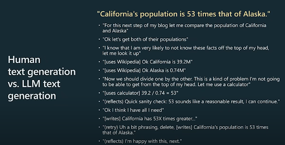
Just finished watching the talk by Andrej Karpathy on the state of LLMs, it's worth the watch for sure and he is so good at clearly communicating intricate details. There is a lot of good stuff that he goes over recording the reward model and reinforcement learning that actually make GPTs or Fine-tuned LLM become chatbots or assistants. However, the one thing I really liked was how he discussed the process of a human generating text vs. an LLM. First, he presents an example of someone trying to respond to a question for a blog post, below is the slide with the steps the person might go through.

https://youtu.be/bZQun8Y4L2A?t=1240

You can see it's pretty complex in terms of all the intricate questions we ask ourselves. Additionally, we rely on resources to improve our knowledge in order to answer the question. This means we understand what we do not know but are able to utilize external resources such as talking with people or searching the internet to update our understanding. When it comes to provided quantitative answers we know that it's likely we will get the math operation wrong so we use other tools, however, we have a good sense of intuition about that qualitative answer, for example, the 53x population factor is plausible given 3 of the largest cities in the USA are in CA. What's more important though is that while we write a response to the question that prompted the blog, we actually introspectively reflect as we write which creates a constant feedback loop with on-the-fly updating.

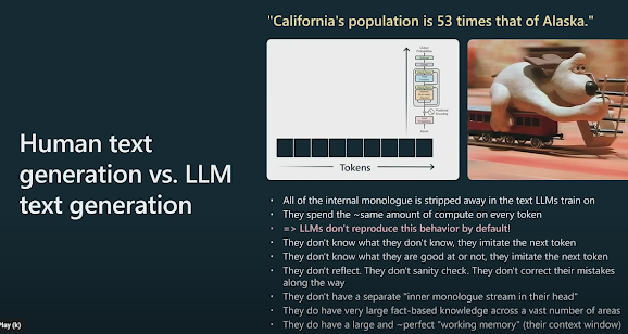
Let's contrast that with what Andrej indicates that LLMs are doing. Remember this is the guy who help founded OpenAI and was an AI lead at Tesla. So I value his insight.

https://youtu.be/bZQun8Y4L2A?t=1360

It's clear from this slide that LLMs don't conduct or possess introspection. What I gathered from his talking over this slide is LLMs are really good at identifying and recalling the context of a prompt and predicting the sequence of tokens/words that would follow. However, they don't really know about their own knowledge or lack thereof, but they are really good at computing the most probably token/text to come next for natural language.

Reuse and Attribution