An op-ed for a new STEM professional degree

I have recently read a few articles about how the Ph.D. process is inadequate in non-academic workforce preparation and how it needs to be revamped. I agree that its time to revamp workforce training, but not necessarily the Ph.D. degree itself. The following post is just my thoughts and opinions, and takes a US and STEM centric focus. I’m just thinking out loud here — not trying to persuade anyone —  so feel free to disagree since I’m interested to hear what others think.

In my opinion it is unfortunate that the Ph.D. degree has been miss represented. The Ph.D. degree is not a degree, in principal, intended to be tailored towards workforce preparation in the same way as professional degrees like a M.D. , J.D., D.D.S, Pharm. D., etc. A Ph.D. is a basic or applied research degree, which means you are being educated on how to expand the knowledge in a given domain by formulating a hypothesis or problem statement and conducting the necessary tasks to provide an explanation or answer. This skill set can be extremely valuable to employers if that is what they are looking for, however, in my opinion many non-academic employers are really looking people who are STEM educated and have a high-level expertise in specific technical skills, which is usually a byproduct of the Ph.D. process. However, I don’t believe a Ph.D. is necessarily the best or only option for this.

I believe a new terminal degree, say we call it Masters (or Doctor) of Technical Skill in ABC, can be established with direct input from non-academic entities. This would be a none-research professional degree.  Something like this probably already exist within a Masters of Engineering or a non-thesis M.S option, but these programs are typically structured around lectures and seminars with minimal practical hands-on training. There is also the obvious issue that most of these kind of programs don’t have modern infrastructures and facilities as well as exist with limited funding levels.

The goal of such programs should be focused on workforce preparation towards becoming an expert in the knowledge, application, modification, and operation of sophisticated software or hardware. From my perspective and background, I could easily see programs such as Masters of Technical Skill in Materials Characterization, whereby students would become extremely skilled in understanding the principals/applications and advance hands-on operation/modification of selected instrumentation, for example SEM, TEM, XPS, Auger, FTIR, Raman, etc. You might argue that this is just a technician degree, but I would argue that these types of systems (or software) require a significant amount of scientific and engineering education prior to becoming a verifiable expert. We can parallel this with how M.D. students after graduation are expected (its more accurate to say required if the person is going practice medicine) to take on a postgraduate residency training program even though they are already highly educated in medicine and life sciences.

Just in materials science and engineering I can imagine several different tracks and sub-focuses. For example,  another program could be a Masters of Technical Skill in Ceramic Synthesis. Students would become highly knowledgeable in powder preparation, green body forming (i.e. relevant wet chemistry), hot isostatic pressing, spark plasma sintering operation, etc. The list can go on and its all about tailoring the program focus towards an industry sectors needs, although to be honest, industry in some cases should be much more specific and realistic about what they are looking for in such students.

The level of training and time will depend on the complicated nature of the skills, systems, or software. I would imagine that the mean time to completion would be around 2-3 years, with some programs probably suitable to be completed in < 2 years. An example of a potentially more challenging program would be Master of Technical Skill in Quantum Computation, here students would have to master both the theory and mathematics of quantum computation/information  and learn about operating and interfacing with complicate hardware.

The two quotes for this post are:

"Education is what remains after one has forgotten what one has learned in school."
– Albert Einstein

"The more that you read, the more things you will know, the more that you learn, the more places you’ll go.” 
– Dr. Seuss

Reuse and Attribution

Simple Example of Entangled States & My Thoughts

Entanglement

In the famous EPR paper, the primary argument is related to the bizarre non-local consequences of entangled quantum states. Einstein's main objection is related to the non-local (spatial) characteristic of entangled states. He suggested that quantum mechanics must be an incomplete theory and argued that our experience in nature appears local. He therefore concluded that hidden variables or additional degrees-of-freedom most likely exist and are not captured by current quantum theory formulations. Unfortunately, well maybe fortunately, Einstein appears to be incorrect about this as exemplified by the work of John S. Bell. The main outcome of Bell's work is that non-local theories can exist without the need for hidden variables and thus entangled quantum states are not restricted by spatial locality. I won't dive to deep into the foundations of quantum theory, but rather just look at a simple mathematical argument for why entangled states exist.

Simple Example

Let me first start with describing a quantum state (i.e. wavefunction) with basis vectors$^*$:

$$|0\rangle = \begin{bmatrix}
1 \\
0
\end{bmatrix} ,\;
|1\rangle = \begin{bmatrix}
0 \\
1
\end{bmatrix}
$$

This is a orthogonal basis set and corresponds to a Hilbert space (abstract function vector space) of $2^n$, where $n$ is the number of particles or objects. Each particle or object can be represented by a linear combination vectors in the Hilbert space. The basis corresponds to that used to describe quantum bits or qubits. 

The basis states can be used to form product basis states, which are given by the tensor product, such that for a system of two objects the  Hilbert space  is $2^2 = 4$ and can be written as:

$$
|00\rangle =\begin{bmatrix}
1 \\
0 \\
0 \\
0 \end{bmatrix} ,\;
|01\rangle =\begin{bmatrix}
0 \\
1 \\
0 \\
0 \end{bmatrix} ,\;
|10\rangle =\begin{bmatrix}
0 \\
0 \\
1 \\
0 \end{bmatrix} ,\;
|11\rangle =\begin{bmatrix}
0 \\
0 \\
0 \\
1 \end{bmatrix} \;,
$$

where the state of a particle/object is represented by a linear superposition of the product basis states, each having a complex amplitude (can be real if the imaginary part is zero). Now we can do something interesting, what if we take the product basis just written above and construct a  potential wavefunction with the following features:

$$ |\Psi\rangle = \frac{1}{\sqrt{2}} \left( |00\rangle + |11\rangle\right).$$

Since we know from that the states $|00\rangle$ and $|11\rangle$ can also be written as product states, as shown above, lets do the following:

$$|\psi_1\rangle = \alpha_1 |0\rangle + \beta_1|1\rangle $$
$$|\psi_2\rangle = \alpha_2 |0\rangle + \beta_2|1\rangle. $$

Now from these definitions lets take the tensor product:

\begin{align}
|\psi\rangle &= |\psi_1\rangle \otimes |\psi_2\rangle \\
 &= \alpha_{1} \alpha_{2} |0\rangle|0\rangle + \alpha_1 \beta_2 |0\rangle|1\rangle + \beta_1 \alpha_2 |1\rangle|0\rangle + \beta_1 \beta_2 |1\rangle|1\rangle \\
 &= \alpha_{1} \alpha_{2} |00\rangle + \alpha_1 \beta_2 |01\rangle + \beta_1 \alpha_2 |10\rangle + \beta_1 \beta_2 |11\rangle .\\
\end{align}

So we now have the given state $|\Psi\rangle$ and the product state $|\psi\rangle$, and if we compare the terms we immediately observe that:

$$\alpha_1 \alpha_2 = \frac{1}{\sqrt{2}} \; \text{and} \;  \beta_1 \beta_2 = \frac{1}{\sqrt{2}}$$

However, since for an orthonormal basis we must have that, $||\Psi\rangle|^2 = 1$ , it then has to be such that:

$$\alpha_1 \beta_2 = 0 \; \text{and} \; \beta_1 \alpha_2 = 0.$$

This would be a contradiction though because its is not feasible  given $\alpha_1 \alpha_2 = \frac{1}{\sqrt{2}}$ and $\beta_1 \beta_2 = \frac{1}{\sqrt{2}}$. We therefore say that quantum state,

$$ |\Psi\rangle = \frac{1}{\sqrt{2}} \left( |00\rangle + |11\rangle\right),$$

represents a quantum entangled state, and cannot be written in terms of product states. Moreover, the determination or expectation of a single particle/object in this entangled state immediately tells us about the state of the other particle/object. For example, if the expectation value of particle 1 is $0.5$ in $|0\rangle$ or $|1\rangle$ then we will know with unity the state of particle 2 is. 

What does it mean

The feature of entanglement is exclusive to quantum mechanics. One way I try to think of things is that quantum states can be composed of two types, those that exist due to the "combination" of quantum states (i.e., product states) and states which manifest as unique quantum solutions which are indecomposable into any other state or description. This fact, of entanglement is one of the great mysteries in quantum physics but its existence is enabling fantastic technologies.

There are two quotes from Niels Bohr's that I think fit well with this post, the first is:

"Einstein, stop telling God what to do [with his dice]!"

-Niels Bohr's, A response to Einstein's assertion that "God doesn't play dice".

This was in response to Einstein's dislike for many of the unexplained conundrums of quantum mechanics. The second quote:

"Anyone who is not shocked by quantum theory has not understood it."

-Niels Bohr's, The Philosophical Writings of Niels Bohr (1987),

Which captures the unexpected and possibly bizarre way of thinking one needs to succumb to in order to appreciate the predictive power of quantum theory (i.e. mathematics and interpretations). Despite this lack of comfort, quantum theories have made extremely accurate predictions and have been validated numerous times through meticulously controlled experiments.

I personally still find the foundations of quantum physics to be nebulous, but this is probably due to my own fallibility. To me its is unsatisfying that we do not not know the true meaning of the wavefunction or more specifically what is the meaning of a Universal wavefunction? Maybe its to complex that we will never know. Then there are questions about why entanglement exist, is it necessary to be consistent with physics as a whole (i.e., General Relativity)? Have we dismissed other understandings to quickly? Does the dendritic many-worlds interpretation originally proposed by Hugh Everett describe reality? What about revisiting non-local hidden variable theories such as Bohmian mechanics (also known as pilot-wave theory and De Broglie-Bohm theory)? How does non-locality make sense, is our notion of space being innate to the universe incorrect? Does space emerge from something else?

All of these question intrigue me, however, I have only scratched the surface  and look forward to learning more about research focused on the foundations of quantum physics. There is a considerable learning curve and start-up time  for me since my formal training is not in theoretical physics, but that won't stop me.

$^*$ The basis vectors are represented using the bra―ket notation pioneered by Paul Dirac. This is a very useful notation but may be unfamiliar to materials science people given that our solid state physics education, to my knowledge, never goes over this because we typically always deal with quantum states (i.e., wavefunctions) in a position or wave-vector basis, for example, $\psi_i(x) = A_i e^{\alpha_i \left(x-x_o\right)^2}$ or $\psi_{k}(x) = \frac{1}{\sqrt{V}} e^{ik\cdot x}$. Therefore the more broad and useful bra―ket notation goes unused.

Reuse and Attribution

Discussion on Quantum States & Corresponding Electrons

My purpose for this blog post is to explore pedagogical approaches to explaining solutions (i.e.  wavefunctions) for the time-independent Schrodinger equation and how electrons are associated with those solutions. In its present form, the blog is not polished and may have erroneous statements, so keep in mind the blog just follows my train of thought. I apologize in advance for confusion or mistakes. For clarity I will try to avoid any gobbledygook (i.e., unnecessary nomenclature).

Quantum States$^\dagger$: A Train of Thought

The first thing to discuss is that we are interested in explaining the motion and interactions of our – humans that is – notion of particles that make up matter. The main confusion is that our intuition/experience tells us to think of the world as particles, however, the whole premise of quantum mechanics is that the motion and interactions cannot be described by classical point particles but rather by "wave-like"$^\mp$ states which are solutions to quantized operators/transformations. It behooves us then to concede that with our current mathematical tools (i.e. equations of quantum mechanics) we are told that the material world, at its smallest scales, is in  "wave-like" states. What does "wave-like" states even mean? It means that the mathematics used to treat the motion and interactions of what we call particles$^\ddagger$ within the theory of quantum mechanics (QM) looks similar to the mathematics used to describe the motion of waves. The difference from the classical picture of waves arises in the nature of the quantum mechanical solutions, that is, the "wave-like" states and their amplitudes exist in a complex number space.

The essence in interpreting the physical meaning of the "wave-like" state solutions, is an additional layer of struggle and falls within the philosophical interpretation of quantum physics. For example what is the meaning of the "wave-like" state if when I interact with the physical world I always observe or measure particles — this is what experiments show us. This bewildering problem still exist even though it has been nearly 100 years since the conception of QM. So why don't we know the meaning? I'm not sure. Its not to say that many great minds haven't proposed insightful ideas, but that there is no clear victor. The most widely accepted and used approach is commonly referred to as the Copenhagen interpretation, which was primarily pushed by Niels Bohr. The main premise is that it is only the magnitude of the complex numbered "wave-like" state that we can assign meaning to as a kind of probability about our [human] intuition of where particles could be. Then there are the many-worlds theory initially proposed by Hugh Everett, pilot-wave theory of David Bohm and De Broglie, and the spontaneous wavefunction collapse theory (GRW). It seems to me that the complexity of trying to explain the philosophical implications of the quantum "wave-like" state is something to admire given that it eludes some of most brilliant of minds. The general theme in physics seems to focus on QM (i.e., wavefunction) predictive description of reality not the inference of its existential meaning.

Okay, lets shift back and think about some examples where waves describe the behavior of a classical physical system. The two most simplest to start with are a vibrating violin string  and drum membrane. In both cases a medium (the string and drum membrane materials) acts as a field — a property given at a point in space, here the property is the elasticity of the material. It turns out that because the string and drum head are pinned down at the edges, only certain characteristic vibrations can exist, these are called modes or in mathematics eigenstates (eigen in German means self/characteristic). The characteristic vibrations are a state that the system (i.e., string or drum head) can exist in, but they do not necessarily always exist, it depends on how the system is excited (i.e. plucked or banged). In many instances the overall vibration of the string or drum head is a combination of characteristic vibrations, an analogy one could think of is how we combine the colors red and green to get yellow. We can combine characteristic vibrations to get a new vibration, this is commonly called linear superposition or combination. 

So now that we've discussed a little about waves, lets revisit the "wave-like" aspect of quantum mechanics. We start by stating that the total motion and interactions of a quantum system is described by a "wave-like" state or wavefunction, $$\Psi\left(\chi_1,\chi_2,\chi_3,\cdots,\chi_N\right)$$,

where $\chi_i$ is a single state function that will depend on position, time, and the type/number of particles.  When the time dependence is removed from the description of the system, that is the system is time-independent, it described by the equation:

$$\hat{H}|\Psi(\chi_i,\cdots)\rangle=E|\Psi(\chi_i,\cdots)\rangle $$

This is the Schrödinger time-independent non-relativistic wave equation which is an eigenvalue problem. Lets describe each term in the equation in  more details. The term $\hat{H}$ is called the Hamiltonian operator named after William Rowan Hamiltonian and describes the dynamics, interactions, and energy components of the system. In Newtonian mechanics we describe a system in terms of the acting forces, in Hamiltonian's representation we use momentum and energy. For a quantum system we can write a generic electronic Hamiltonian as,

\begin{align}
H &= K.E. + P.E. \\
&=\frac{-\hbar}{2m_e}\sum_{i}^{N}\nabla_{i}^2+\frac{1}{2}\sum_{i,j}^N V(\mathbf{r}_i,\mathbf{r}_j)
\end{align}.

The first term representing kinetic energy (momentum) and potential energy (field interactions). In this representation the K.E. and P.E. are said to be operators — I tend to think of these as being equivalently equal to transformations —  that are "quantized" in their representation. These operators act on the "wave-like" state, $\Psi$, of a system producing a representation of the system in terms of K.E. and P.E. At this point the representation is a linear combination of characteristic "wave-like" states that the system could be in.

But what happens if I ask the question "What energy is associated with a particle in a given state and where can that particle be in physical space?", more specifically what can I know about the particle that makes sense or has meaning to me, the human. See at this point we just know a spectrum of energies associated with the "wave-like" solution states, which doesn't have a clear comprehensible meaning to us/me yet. It is at this junction where the "reality" of outcomes of Q.M. falls in the the realm of philosophical physics, or in other words, subjected to interpretation. In quantum physics pedagogy the stance is we need to make an expectation or guess on what the outcome is to be. To do this we say we have to project/collapse/measure the "wave-like" states onto a known meaningful platform, a set of states, to get a understanding of where a particle might be. It turns out that this projection is best interpreted as information about the probability or probability of transition of  "wave-like" state; that is with respect to the state its in and the state I know. This is typically what is understood as the expectation value or measurement collapse argument (also more commonly called the Copenhagen interpretation), which is necessary for us (humans) to relate the math or experimental results of quantum mechanics to our notion of particles. To write this out we would have:

$$ <\Psi|H|\Psi> = E <\Psi|\Psi> $$

I use this equation to try and understand the measurement outcome in quantum experiments, that is, the act of observing in an experiment is akin to enforcing a projection onto a known state/solution.

So lets recap, we mentioned that quantum systems can be treated mathematically similar to wave dynamics. We said that these quantum systems have characteristic "wave-like" solutions, e.g., eigenvalues and eigenvectors. Then an equation relating the operation on or transformation of the quantum "wave-like" state resulted in the same state multiplied by the eigenenergies, but we said it only tells us about the energy spectrum and the states the quantum system could be in. Finally, we tried to understand this by projecting or collapsing the "wave-like" solutions onto known solutions (I forgot to mention these could initial states we used prior to applying any operators or transformations).

All this discussion has so far abstracted the "wave-like" states from actual matter that occupies the states. This is akin to our string or drum which we known has vibrating solutions regardless of if its actually been plucked or banged. The next step is to understand how our notion of particles or matter is associated with the "wave-like" states. In other words, how particles or matter can occupy those solutions. It turns out that electrons, which are the basic building blocks for how we (humans that is) experience chemistry and materials, have very specific rules for how they assume a given state. Electrons are indistinguishable particles, meaning they cannot be individual tracked or resolved,  but they have a unique property associated with the "wave-like" state that requires them to take on a specific intrinsic angular momentum which is called spin$^\star$. This spin characteristic gives rise to "wave-like" states such that only a single electron is allowed to acquire a give "wave-like" state of specified spin. In QM this is called the Pauli exclusion principal for fermions which was postulated by Wolfgang Pauli based on spin-statistics theorem. It wasn't till Paul Dirac's work with relativistic QM of an electron that "spin" was deduced to be a consequence of the inclusion of Einstein's special relativity, at least this is my understanding of the outcome of the Dirac Equation.

So now let me try and give analogy to re-explain this, not sure it will work out.

The Race Track (Quantum) Architect

We start our conceptual  understanding of a quantum system which describes electrons in an environment of atomic nuclei.

A quantum architect is told that they will need to design a race track. The race track has several constraints in how it can be built. The first piece of information the architect is given is where the race track will be built. This will dictate the shape, number of bends and slopes of the race track. The race track terrain is our analogy for the potential energy surface created by the combinatoric interactions among the atomic nuclei and electrons.

We then tell the quantum architect how many lanes/tracks are needed to accommodate the drivers, these are our analogy for the "wave-like" states an electron can be in. There are additional pieces of information we need to tell our architect about this race track, that is, the drivers of this race track have unique characteristics. The first is that they all look identical and drive the same car, so we cant tell them apart, therefore we never know who is really in each lane. The next unique characteristic is that each driver has a preferred direction (spin) of driving, forward or reverse, and preferred lane (spatial location). The third characteristic is that each driver dislikes all other drivers, so they try to avoid each other at all costs and never use the same lane, with one exception, that is when two drivers who drive in opposite directions use the same lane/track they both usually perform better — we will take this to mean lower energy — but no lane can ever accommodate drivers who are moving in the same direction.

So lets break down our analogy. The number of lanes corresponds to the number of "wave-like" state solutions we can have which depends on the type of system we are interested in; here the system is our race track configuration based on the number of drivers, terrain, etc. The fact that all the drivers look identical and drive the same car is a characteristic of electrons, they are indistinguishable particles. The preferred driving direction of each driver corresponds to a innate property of electrons (more broadly fermions) dubbed "spin", where its value corresponds to a positive (up) or negative (down) sign due to its behavior in magnetic fields. The fact that the drivers dislike each other but can have special configurations in the lanes corresponds to the Coulomb and exchange forces, where the latter is due to spin and the Pauli exclusion principal.

With all this information the architect is ready to build our race track, but, we through in an additional caveat, that we need him/her to build it in such a way that the number and shape of the lanes can change dynamically. At this point he/her is annoyed, but says their company is so skilled that they can dynamically adjust the state of the race-track to accommodate any number of drivers. So now drivers can be added or removed from the rack track simply by the architects ability to add or remove lanes.

Okay, so we have described the quantum state of electrons using an analogy.  I'm not sure how good this was but I will continually revisit it to improve. No quote for this blog given it is not final.

$^\dagger$ Please comment if you find any explanation of analogy incorrect. This blog post was a result in trying to explain to my wife, who is not trained in a STEM field, the physics that gives rise to the chemical and material world around us. What inspired this was my reading of books discussing self-learning approach dubbed the Feynman technique, pioneered by the famous physicist Richard Feynman. The idea is you take a topic or idea that your familiar with but not sure your level of understanding and work through the topic/idea (e.g. Quantum States) as if you were teaching it to someone else. The purpose is to help identify areas where you may lack understanding or capability (i.e. mathematics). Since I'm always trying to improve my level of knowledge in quantum mechanics, this blog post was my attempt to do so.

$^\mp$ I have chosen to use the quoted term "wave-like" instead of the more common and probably accurate term wavefunction. My reason for doing so is at this level of discussion I don't think any additional clarity is gained by using the word wavefunction, but "wave-like" in my opinion, conveys that the wavefunction will have a functional form that is reminiscent of a wave or wave packet. Anyhow, I will use the two interchangeably throughout this blog.

$^\ddagger$ My understanding is that the leading view in quantum (field) physics is that particles are a manifestation of excitations in quantum fields. In other words, it is quantum fields that exist not particles, and when we speak of particles, say an electron, we are just talking about quantized excitation in an electron field.

$^\star$ The origin of the term spin is unfortunate because it forces a physical picture of the electron which isn't necessarily true in the framework of QM. It comes from the initial view that an electron is not a structure-less point object in space, but that it has some diameter/volume  associated with it and spins about its own axis (as the earth does). To my knowledge the diameter of a electron has never been observed or measured. As mentioned in the main text, the spin is a result of special relativity which adds chirality (handedness) to the spatial part of the wavefunction, also called a spinor.

Reuse and Attribution

Atomic View of Thermal Expansion

To discuss how thermal expansion emerges in materials one can start with a simple view of the potential energy between atoms. Let us first look at the potential curve as function of separation, $R=||\bf{r}_1 - \bf{r}_2||$, between two atoms as shown in the figure below:

In the figure the equilibrium bond distance between two atoms is indicated by the minimum in the potential energy. In a system where the thermal energy is not dominant (i.e., low temperatures) the potential energy can be approximated harmonically, and therefore the displacements, $\Delta r = (r -r_{eq})$, due to the forces will be symmetric in an averaged sense. This is highlighted in the figure inset showing that the harmonic (blue) matches well with the potential curve for small $\Delta r$.

When the thermal energy in the system begins to become significant, the harmonic approximation is no longer appropriate and the displacements are non-symmetric about the equilibrium bond distance. This asymmetry gives rise to thermal expansion of a material. This is further shown in the inset with the anharmonic curve (red) showing better agreement with the potential curve than the harmonic at larger $\Delta r$.

The atomic view of thermal expansion manifest in bulk through the isotropic (i.e. volumetric) thermal expansion of a material which is given by the coefficient of thermal expansion,

$$\alpha = \frac{1}{V}\frac{\partial V}{\partial T}_P $$

where $V$ is the volume, $T$ the temperature, and $P$ indicates the derivative at constant pressure. It is also common to refer to this as the coefficient of thermal expansion (CTE).  

The quote for this post is:

Science knows no country, because knowledge has no identity, and therefore exist to illuminate the world.
-Louis Pasteur (modified)

References

[1] The Materials Physics Companion, IoP, 1st ed., A.C. Fischer-Cripps.

Reuse and Attribution

Lagrange Multipliers

In science and mathematics it is very common for the need to determine the local extrema of a function, $f(x,y,z,\cdots)$ subject to some constraint. If the constraint (function), which depends on same set of independent variables, can be expressed as $h(x,y,z,\cdots) = 0$, then one can rewrite a new constrained function as:

$$ g\left(x,y,z,\cdots,\lambda \right) = f\left(x,y,z,\cdots\right) + \lambda h\left(x,y,z,\cdots\right).$$

The variable $\lambda$ is known as the Lagrange multiplier. The condition for an extrema (i.e., minima or maxima) occurs when the partial derivatives are zero, more explicitly:

$$\begin{align}\frac{\partial g}{\partial x} &= \frac{\partial f}{\partial x} - \lambda \frac{\partial h}{\partial x} = 0 \\\frac{\partial g}{\partial y} &= \frac{\partial f}{\partial y} - \lambda \frac{\partial h}{\partial y} = 0  \\ \vdots \\\frac{\partial g}{\partial \lambda} &= \frac{\partial f}{\partial \lambda} - \lambda \frac{\partial h}{\partial \lambda} = 0,\end{align}$$

with the last term $\frac{\partial g}{\partial \lambda} = h(x,y,z) =  0$. This sets up our system of equations that can be solved algebraically. To provide some additional context, this approach is used in areas such as thermodynamics and machine learning (more commonly referred to as regularization). The more general form of the function $g$ when several constraints are used is given by the Lagrangian function:

$$ \mathcal{L}\left(x,y,z,\cdots,\{\lambda\}\right) = f\left(x,y,z,\cdots\right) + \sum_i \lambda_i \, h_i\left(x,y,z,\cdots\right) $$

Lets see the use of Langrange multiplier in action with a simple example, a parabola constrained by a circle. Our function, $g(x,y) = 10x^2 - 5y$, and our constraint is $h(x,y) = x^2 + y^2 -1$.  Writing the new function $h(x,y,\lambda)$,

$$ h\left(x,y,\lambda\right) = 10x^2 - 5y + \lambda(x^2+y^2-1) $$

Now working through the partial derivatives of $h(x,y,\lambda)$:

$$\frac{\partial g}{\partial x} = 10x+\lambda(2x) = 0$$
$$\frac{\partial g}{\partial y} = -5 +\lambda(2y) = 0$$
$$\frac{\partial g}{\partial \lambda} = x^2+y^2-1 = 0$$

We now find the Lagrange multiplier, $\lambda$, using the first equation,

$$\begin{align}
2x(10+\lambda) &= 0 \\
\lambda &= -10
\end{align}
$$

we can calculate $y$, with the second equation,

$$\begin{align}
-5-10*(2y) &= 0 \\
y &= -0.25
\end{align}
$$

and with the constraint equation we can find $x = 0.9862$. This example is very simple and does not demosntrate the full power of Lagrange multipliers, which is extremely powerful in multivariate calculus. The quote for this blog post is by Joseph-Louis Lagrange himself:

"I regard as quite useless the reading of large treatises of pure analysis: too large a number of methods pass at once before the eyes. It is in the works of applications that one must study them; one judges their ability there and one apprises the manner of making use of them"
- Joseph-Louis Lagrange

References & Additional Reading

[1] Advanced Engineering Mathematics, Wiley, 8th ed., E. Kreyszig.

[2] The Mathematics Companion, IoP, 1st ed., A.C. Fischer-Cripps.

[3] Thermodynamics in Materials Science, Robert DeHoff, 2nd ed.

Reuse and Attribution

Ferroelectric Response

The spontaneous electric polarization in response to an externally applied electric field is what is referred to as ferroelectricity. The electric polarization, $P$, in most cases is proportional to the applied electric field. For review the polarization is give by:
\begin{align}
\mathbf{P} &= N\mathbf{\mu}_{D} = \alpha \mathbf{E} \\
\alpha &= \alpha_{e^{-}}+\alpha_{ion}+\alpha_{mol}
\end{align}
where $N$ is the dipole number density. The polarizability coefficient is contribution from electric, ionic, and molecular dipoles.

When the response is linear the material is classified as being dielectric, elsewise its referred to as being paraelectric. The paraelectric behavior is strongly tied to temperature and disappears at the Curie temperature ($T_c$). When a spontaneous remanent electric polarization occurs upon removal of an applied electric field the material is termed ferroelectric; these materials show typical hysteresis behavior.

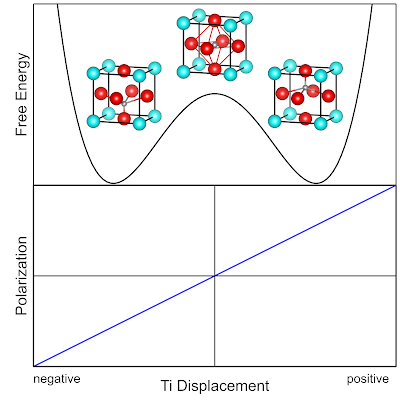
One of the most ubiquitous materials that shows ferroelectric behavior is Barium Titanate ($\text{BaTiO}_3$). The $\text{BaTiO}_3$ crystal has a Tetragonal unit cell, i.e. all angles are 90 degrees but only two sides have the same length ($a=b\neq c$). The species tend to be predominately in an ionic electronic structure configuration, i.e., species at the lattice sites behave like anions and cations. The $\text{Ti}^{+4}$ cation in $\text{BaTiO}_3$ sits in the center of the unit cell and can occupy several slightly off center positions that give rise to a static permanent electric dipole moment. In the illustration below the free energy profile, unit cell with Ti displacement (grey atom) and the change in electric polarization is qualitatively shown.

Illustrative profiles of free energy and electric polarization for BaTiO3 (Perovskite structure, #221 Pm$\bar{3}$m, when no spontaneous polarization occurs). The spontaneous polarization is due to displacement of the Ti center which lowers the free energy of the system.

At temperatures above the Curie temperature each unit cell has a randomly oriented electric dipole moment and thus no bulk permanent moment. Below the Curie temperature the exchange interactions between the individual electric dipole moments will cause some preferred orientation.  The Curie temperature for several ferroelectric materials is listed in the table below:

Material	Curie Temperature [K]
α-Fe	1043
PbTiO3	763
PbZrO3	506
BaTiO3	400
NaNbO3	336
ZnTiO3	278
NH4H2PO4	148

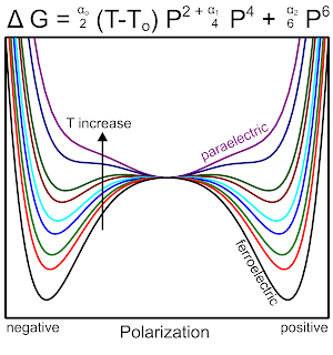
The change in free energy as a function of spontaneous polarization and temperature follows a double well potential typically given by the Ginzburg-Landau theory. The result is a free energy expression written in terms of expansion coefficients that capture the materials spontaneous polarization while accounting for crystal/anisotropy effects. An example of temperature dependence is given below highlighting that at elevated temperatures the spontaneous polarization is weak and therefore polarization is dominated by a paraelectric response.

Free energy as a function of polarization and temperature, illustrative example showing how a material transitions from ferroelectric to paraelectric.

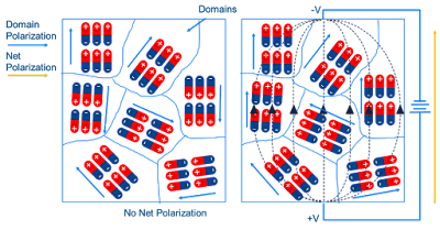
Spontaneous alignment (i.e. no external field) of neighboring unit cell dipole moments will eventually lead to the formation of domains which can have length scales beyond several nanometers. The formation of these domains is the typical criteria for classifying a material as being a ferroelectric The illustration below pictorially shows such phenomena,

Example of domain polarization and external field induced net polarization (image adapted from https://ec.kemet.com/dielectric-polarization)

In the presence of an applied external electric field, the individual domains can will be driven to align with the field direction as to minimize the free energy, $ G = P_{i}E_{i}$. One can also write the difference in free energy, $\Delta G$, due to changes in the domain orientation such that:
\begin{align}
\Delta G &= G_{P_1} - G_{P_2} \\
&= \Delta P^s E_{i} + \frac{1}{2} \Delta \chi_{ij} E_i E_j
\end{align}
in the expressions above we use $i,j,\cdots$ tensor notation (a.k.a Einstein summation) to indicate coordinates. The term $P^s$ is the spontaneous polarization term and $\chi_{ij}$ susceptibility tensor.  The $\Delta$ in front of the material parameters indicates the difference in values between the two states. The change in free energy drives the domains so that they both align and spatial grow until a saturation condition is meet. The change in domain structure has lowered the configurational entropy and "poled" domain structure no longer remembers the initially random polarization configuration. This leads to a a hysteresis curve, where upon reversal of the applied electric field a different polarization configuration is sampled. I will have a blog on hysteresis phenomena.

The quote for today is an excerpt from one of the original documents highlighting the discovery of electric polarization and piezoelectric effects in a mineral salt (Rochelle salt):

"It appears then, that the asymmetry of the throws in Anderson's experiment is due to a hysteresis in electric polarization analogous to magnetic hysteresis. This would suggest a parallelism between the behavior of Rochelle salt as a dielectric and steel, for example, as a ferromagnetic substance."
- Joseph Valasek, APS Minutes, 1920

References & Additional Reading

[1]  Properties of Materials: Anisotropy, Symmetry, Structure , Robert E. Newnham, 1st ed.

[2] Thermodynamics in Materials Science, Robert DeHoff, 2nd ed.

Reuse and Attribution

Ideal Solution Mixing: A-B Lattice

Here we will review the ideal solution mixing model for simple A-B lattice random mixing alloy system. The first step is to recall that for any system (e.g. state or phase) we can write the Gibbs free energy as:

$$ G = H-TS $$

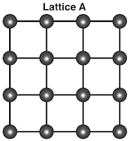
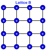
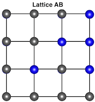
where $H$ is the enthalpy, $T$ the temperature, and $S$ the entropy. We now propose that we have two isolated systems, lattice A and lattice B, and we want to find the change in Gibbs free energy when the two are combined to form a lattice with both A and B sites (randomly). An illustrative example would look something like below.

The next step is to write the change in Gibbs free energy as:

\begin{align}
\Delta G^{mix} & = G_{initial} - G_{final} \\
& = \Delta H^{mix} - T \Delta S^{mix} \\
\end{align}
Notice that we are using the label $mix$ to indicate that the change in Gibbs free energy is due to the mixing of the two lattices into one (i.e. Gibbs free energy of mixing).

In the ideal solution mixing model, we first approximate that $\Delta H^{mix}$  is negligible and taken to be zero. We can think of this as meaning that we assume no change in internal energy due to the chemical interactions between A and B. The next assumption is that the change in entropy is strictly due to configurational arrangement of A and B points on the combined lattice. This means that entropic effects due to lattice vibrations or magnetic ordering are not accounted for. Thus the Gibbs free energy has a simple relation to entropy:

$$ \Delta G^{mix} = - T \Delta S^{c} $$

The next step is to define the representation for the configurational entropy. To do this we will use to facts that each microstate is probabilistic and given by the combinatorics (i.e. possible configurations ). This is compactly represented by the famous equation:

$$ S^{c} = k_b \ln \omega^{c} $$

with $k_b$ being the Boltzmann constant and $\omega^{c}$ the configuration combinatorics. For the lattice AB this is going to be given by:

$$ \omega^{c} = \frac{N!}{N_{A}!N_{B}!}$$

where $N=N_{A}+N_{B}$ and $N_{A}$ and $N_{B}$ are the number of sites of a given type. At first glance calculating the configurational entropy may not seem daunting, however, logarithms of factorials can become demanding to calculate very quickly. Fortunately enough there is an approximation provided by mathematician James Stirling that allows one to approximate logarithms of factorials and is given by:

$$ \ln N! \approx N \ln N - N $$
Using this approximation we can determine $\omega^{c}$ and distill the expression of $S^{c}$ into something that is relative compact and meaningful. Apply the approximation we get:
\begin{align}
 \ln \omega^{c} &= N \ln N - N - \left[\ln\left(N_{A}!N_{B}!\right)\right] \\
&= N \ln N - N - \left[ N_{A} \ln N_{A} - N_{A} + N_{B} \ln N_{B} - N_{B}\right] \\
&= N \ln N - N_{A} \ln N_{A} - N_{B} \ln N_{B} - N + N_A + N_B \\
\end{align}
The last three terms cancel out, e.g., $N_A + N_B = N$ and we then rewrite the first term as:
\begin{align}
\ln \omega^{c} &= \left(N_A + N_B\right) \ln N  - N_{A}\ln N_A - N_{B}\ln N_B \\
&=-\left[N_A \ln \left(\frac{N_A}{N}\right) + N_{B}\ln\left( \frac{N_B}{N}\right) \right]
\end{align}
the ratio of $X_A = \frac{N_A}{N}$ or $X_B = \frac{N_B}{N}$  are the fraction of sites on the mixed lattice with A and B sites, respectively. Let us take one further step by multiplying the equation above by $\frac{N}{N}$ to get
$$ \ln \omega^{c} = -N \left[ X_A \ln X_A + X_B \ln X_B \right] $$
Now we can write $\Delta S^{mix}$ as,
$$ \Delta S^{mix} = -k_{b} N \left[ X_A \ln X_A + X_B \ln X_B \right] $$
if we assume that the total number of N sites on the alloy lattice is comparable to the number of particles in 1 mole, i.e., Avogadro's number $N_a = \text{6.022}\times \text{10}^{\text{23}}$, then we can write the Gibbs free energy of mixing in most familiar form as:
\begin{align}
 \Delta G^{mix} &= -T \Delta S^{mix} \\
&= -T \cdot -k_{b} N_{a} \left[ X_A \ln X_A + X_B \ln X_B \right]  \\
&= \boxed{RT \left[ X_A \ln X_A + X_B \ln X_B \right]}
\end{align}
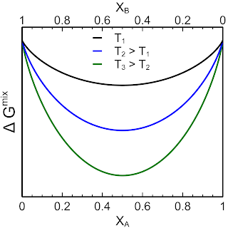
where $R$ is the gas constant given by  $k_b N_a$. We can get a sense for how the Gibbs free energy of mixing changes with temperature as shown in the graph below,

From the graph we observe two features, 1.) the Gibbs free energy of mixing for an ideal solution is a symmetric function, 2.) as the temperature is increased $\Delta G^{mix} is decreases. Not that in the graph the line(s) do not extend to zero and one, this is because these would be given by the Gibbs free energy of the reference states of lattice A and B.

Ideal solution mixing is typically not suitable for real material alloy systems and thus other approximations such as the regular solution model are used. In the regular solution model we use the same $\Delta S^{mix}$ and include a non-zero expression for $\Delta H^{mix}$. The most accurate approach for calculating Gibbs free energy of mixing for real materials is to use CALPHAD methodologies.

For this blog postings quote we will get two quotes:

"Nothing in life is certain except death, taxes and the second law of thermodynamics."
-Seth Lloyd, MIT Professor 

"In this house, we obey the laws of thermodynamics!"
-Homer Simpson, response to Lisa's perpetual motion machine

References & Additional Reading

[1] Thermodynamics in Materials Science, Robert DeHoff, 2nd ed.
[2] Introduction to the Thermodynamics of Materials, D.R. Gaskell, 5th ed.

Reuse and Attribution

Exact Differential Equations

The general form of a first-order differential equation is given by the following:

$$ M(x,y)dx + N(x,y)dy = 0$$

our differential equation is said to be exact if it satisfies the following exactness test:

$$\frac{\partial M\left(x,y\right)}{\partial y} = \frac{\partial N\left(x,y\right)}{\partial x}$$

The goal is to determine a function $f(x,y)$ that satisfies the following:

$$df = M(x,y)dx + N(x,y)dy$$

$$ \frac{\partial f\left(x,y\right)}{\partial x} = M\left(x,y\right)$$

$$ \frac{\partial f\left(x,y\right)}{\partial y} = N\left(x,y\right)$$

Let us look at the following example differential equation:

$$\left(y^{2}-2x\right)dx + \left(2xy+1\right)dy=0$$

Taking the partial derivatives of the functions corresponding to $M\left(x,y\right)$ and $N\left(x,y\right)$, we get:

$$ \frac{\partial M}{\partial y} = 2y $$

$$ \frac{\partial N}{\partial x} = 2y $$

So our differential equation is indeed exact and we now can find the total function, $f(x,y)$, whose derivative is equal to our differential equation. This is done by integrating  the functions $M\left(x,y\right)$ and $N\left(x,y\right)$,

$$M\left(x,y\right) = \frac{\partial f\left(x,y\right)}{\partial x}$$

$$f = \int{\left(y^{2}-2x\right) dx} = xy^{2}-x^{2} $$

similarly for $N\left(x,y\right)$,

$$N\left(x,y\right) = \frac{\partial f\left(x,y\right)}{\partial y}$$
$$f = \int{\left(2xy+1\right)dy} = xy^{2}+y $$

In both cases, we ignore the constant of integration. We now can identify unique terms and construct the function, $f(x,y)$, by summing these terms:

$$f\left(x,y\right) = xy^{2}-x^{2}+y=\text{constant}$$

So we have identified a function, $f\left(x,y\right)$, that is a solution to our exact differential equation.

Now for our quote:

I became an atheist because, as a graduate student studying quantum physics, life seemed to be reducible to second-order differential equations. It thus became apparent to me that mathematics, physics, and chemistry had it all and I didn't see any need to go beyond that.
-Attributed to Francis Collins but unconfirmed.

Reuse and Attribution

Matrices

A matrix is an array of numbers arranged with $m$-rows and $n$-columns. When $m=n$ the matrix is termed square. The index of an element in a matrix is notated using the indices $i$ and $j$ for the rows and columns, respectively. For example:

$$\mathbf{B}=
\begin{bmatrix}
b_{11} & b_{12} \\
b_{21} & b_{22} \\
\end{bmatrix}.
$$

The algebra of matrices is straightforward, for example, addition occurs by adding same indexed elements:

$$\mathbf{B}+\mathbf{C} =
\begin{bmatrix}
b_{11}+c_{11} & b_{12}+c_{12} \\
b_{21}+c_{21} & b_{22}+c_{22} \\
\end{bmatrix}
.$$

We can write the addition operation in more compact form using implicit index notation, e.g., $\mathbf{B}+\mathbf{C}=b_{ij}+c_{ij}$. Keep in mind that the dimensions of the matrices must be the same for addition or subtraction operations.

Multiplication of matrices by a scalar quantity is simply, $S\cdot\mathbf{B}$. When multiplying two matrices, the inner dimensions must be the same, for example, if $\mathbf{B}$ is a $m \times n$ then $\mathbf{C}$ must be a $n \times p$. In other words, the number of columns in $\mathbf{B}$ must be equal to the number of rows in $\mathbf{C}$. The operation is written in compact as follows:

$$ c_{jk} = \sum_{i=1}^{n} a_{ji}b_{ik}.$$

Here are some examples, $c_{11} = a_{11}b_{11}+a_{12}b_{21}$ and $c_{12} = a_{11}b_{12} + a_{12}b_{22}$. An important operation/transformation of matrices is the transpose, which is the process of switching elements in the rows and columns. The transpose is indicated with a superscript capital "T", e.g., $\mathbf{B}^T$. For a square matrix, the diagonal components are commonly referred to as the principal terms and the sum of them is the trace of the matrix. For square matrices that have ones as diagonal terms and zeros as off-diagonal terms, we refer to them as unit of identify matrices, for example:

$$\mathbf{I}=\begin{bmatrix}
1 & 0 & 0 \\
0 & 1 & 0 \\
0 & 0 & 1 \\
\end{bmatrix}.$$

Identity matrices are commonly represented with $\mathbf{I}$. Another important property of square matrices is invertibility. A matrix is said to have an inverse if it satisfies the following condition:

$$\mathbf{A}\mathbf{B} = \mathbf{I},$$

we call $\mathbf{B}$ the inverse of $\mathbf{A}$. If a square matrix doesn't have an inverse it is referred to as singular. Matrices that have the inverse which satisfies the condition:

$$\mathbf{A}^{T}\mathbf{A}=\mathbf{I},$$

are orthogonal matrices. A determinant is a specific value that can be computed for square matrices and can be thought of as the scaling factor for linear transformations. The determinant is typically written as:

$$\text{det}\, \mathbf{B} = \Delta \mathbf{B} = |\mathbf{B}|,$$

For 2x2 matrices the determinant is determined by taking the product of the diagonals and subsequent difference between them, as shown below:

$$|\mathbf{B}| =
\begin{vmatrix}
b_{11} & b_{12} \\
b_{21} & b_{22} \\
\end{vmatrix} = b_{11}b_{22}-b_{21}b_{12}.$$

Another method for finding the determinant is using the Laplace expansion method. Determinants have the following commuting properties:

$$|\mathbf{A}\mathbf{B}| = |\mathbf{A}||\mathbf{B}|,$$
$$|\mathbf{A}| = |\mathbf{A}^{T}|.$$

A matrix that is singular will have a determinant that evaluates to zero, thus this is a good way for identifying if a matrix has an inverse.

Matrices and determinants are an important component to the field of  linear algebra, so having good command over them is a serious advantage. I know there are a lot of keywords presented in this post that were not given a formal mathematical description but I strongly suggest clicking the link and reading on to get a better sense of there use in linear algebra.

For this post we will provide a quote from a mathematician who did a lot of research in advance algebra and group theories.

"We [Kaplansky and Halmos] share a philosophy about linear algebra: we think basis-free, we write basis-free, but when the chips are down we close the office door and compute with matrices like fury."
-Irving Kaplansky, Paul Halmos: Celebrating 50 Years of Mathematics

References & Additional Reading

[1] Advanced Engineering Mathematics, Wiley, 8th ed., E. Kreyszig.

[2] The Mathematics Companion, IoP, 1st ed., A.C. Fischer-Cripps.

Reuse and Attribution

Brittle Fracture & Dislocations

Before I dive right into dislocations, let me provide a quick refresher on brittle fracture. From a theoretical perspective, crystalline materials are perfectly repeating spatial structures that lack any defects to disrupt their symmetry. These perfect structures should behave completely elastic, i.e. spring-like, until the onset of fracture due to bond breaking.

Prior to fracture the elastic regime of a crystal's response to loading can be described by anisotropic/isotropic version of Hooke's law : $\sigma_{ij} = C_{ijkl}\epsilon_{kl}$ where $\sigma_{ij}$ is the stress tensor, $\epsilon_{kl}$ is strain tensor, and $C_{ijkl}$ is the stiffness tensor. To describe what happens after the elastic region we require a model for immediate fracture, i.e. fracture occurring at the speed of sound in a material. This event is more commonly referred to as brittle fracture. The most simple model for near perfect brittle fracture is given by the Griffith's criteria. This criteria is based on the stress required to break all the bonds between two atomic planes in order to create a free surface. Typically, the Griffith's criteria is more generally discussed in terms of the stability of a crack with a given length, $l$. For tensile loading, the condition for fracture is given by the equation:

$$ \sigma_{fracture} = \sqrt{\frac{2 E \; \gamma}{\pi \;l}} $$

where $E$ is the Young's modulus , $\gamma$ the surface energy, and $l$ the surface (or crack) length. Therefore, a prototypical brittle material should fracture when $\sigma_{fracture} \leq \sigma_{applied}$. In most cases this is a poor approximation including brittle ceramics, which one might suspect would fit the criteria. The table below provides a few examples of calculated fractured stress for a 0.05 mm crack length of different materials.

Material	$\sigma_{fracture}$[MPa]	E [GPa]	$\gamma$ [mJ/m$^2$]
Silicon	51.6	169	1240
Silica Glass	17.2	75	310
NaCl	12.3	40	300
MgO	61.6	1200	249
CaCO3	15.3	230	80

So why don't metals and engineered materials have brittle fracture characteristics, for example, gold. This is because nature (or man) introduces imperfections into materials that give rise to behavior which deviates from perfect elastic-to-brittle fracture, we call this plasticity meaning non-reversible/permanent deformation.  One major contribution to plasticity are planar defects termed dislocations, these are extra atomic planes that are squeezed in between the parent crystal lattice. In the image below, an example of an edge dislocation is shown.  The dislocation core occurs on the slip plane, i.e., the atomic plan where the dislocation can move about.

Example of a line dislocation with the core marked by the perpendicular symbol. The dashed blue line indicates the slip plane, i.e., the plane for which the dislocation can glide along when a shear force is applied. Once the dislocation reaches a surface it generates a step. Not shown is the burgers vector (adapted from structuredatabase.wordpress.com).

One of the consequences of squeezing extra atomic planes in a host crystal, is the incipient strain/stress fields around dislocations and as a result of this, applying an external load provides enough energy for the dislocation to glide. Dislocations therefore have a mobility associated with them due to these strain/stress fields. This mobility occurs by glide motion along certain atomic planes with a given direction. This magnitude and direction is characterized by the Burgers vector, named after the Dutch physicist, Jan Burgers. For a closed-pack lattice, the magnitude of the Burgers vector along directions $h$,$k$,$l$ (see Miller indices notation post) can be calculated as:

$$ ||\mathbf{b}|| = \frac{a}{2}\sqrt{h^2+k^2+l^2}$$

In association with the Burgers vector is the Burgers circuit, which characterizes the vector magnitude and direction by comparing to a perfect crystal to a dislocation containing crystal.

A complete Burgers circuit for a perfect crystal (left) and the burgers circuit for edge (top-right) and screw (bottom-right) dislocations. As you can see the burgers vector is the extra segment that goes beyond the length of the perfect circuit (adapted from wikipedia)

A perfect example of plasticity induced by dislocations is when a piece of metal is subjected to a shear force. Rather than fracture, as prescribed by Griffith's criteria, dislocations will absorb the applied energy and subsequently move, thereby resulting in plastic or irreversible deformation. In the image shown below produced by Y.-T. Zhou et al. using HRTEM [2], the authors show nicely an edge dislocation in a MnS inclusion inside a steel matrix.

(a) Bright field TEM image of the dislocation distribution in a MnS inclusion. (b) An HRTEM image of the dislocation core. By drawing a closure surrounding the core, the Burgers vector of the dislocation is determined as $\frac{a}{2}[\bar{1}10]$ (figure and caption adapted from ref. [2])

If you would like a more through background on brittle fracture and dislocation dynamics I suggest the text by W.D. Kingery et al. [3] and V. Bulatov and W. Cai [4], respectively. I particularly like the V. Bulatov and W. Cai book since it has excellent exercises to work on. There are also books by Hirth and Lothe and Hull and Bacon focused on introduction to dislocation theory. Now for the selected quote:

“You have to know something to learn something”
-W. David Kingery,  father of modern ceramics, quoted by D. Uhlmann and P. Vandiver

References

[1] The Materials Physics Companion, IoP, 1st ed., A.C. Fischer-Cripps.

[2] Y.-T. Zhou, et al., Philos. Mag. (2015). doi:10.1080/14786435.2015.1052030
[3] Computer Simulations of Dislocations, Oxford Series on Materials Modeling, 1st ed., V. Bulatov and W. Cai
[4] Introduction to Ceramics, Wiley-Interscience, 2nd ed.; W.D. Kingery, H.K. Bowen, D.R. Uhlmann

Reuse and Attribution