Search Blogs

Thursday, June 20, 2019

Ferroelectric Response


The spontaneous electric polarization in response to an externally applied electric field is what is referred to as ferroelectricity. The electric polarization, $P$, in most cases is proportional to the applied electric field. For review the polarization is give by:
\begin{align}
\mathbf{P} &= N\mathbf{\mu}_{D} = \alpha \mathbf{E} \\
\alpha &= \alpha_{e^{-}}+\alpha_{ion}+\alpha_{mol}
\end{align}
where $N$ is the dipole number density. The polarizability coefficient is contribution from electric, ionic, and molecular dipoles.

When the response is linear the material is classified as being dielectric, elsewise its referred to as being paraelectric. The paraelectric behavior is strongly tied to temperature and disappears at the Curie temperature ($T_c$). When a spontaneous remanent electric polarization occurs upon removal of an applied electric field the material is termed ferroelectric; these materials show typical hysteresis behavior.

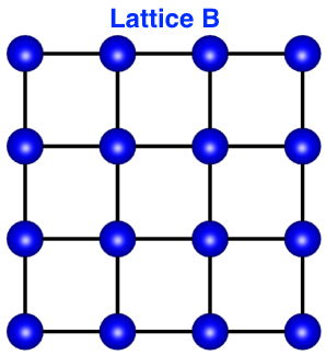
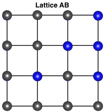
One of the most ubiquitous materials that shows ferroelectric behavior is Barium Titanate ($\text{BaTiO}_3$). The $\text{BaTiO}_3$ crystal has a Tetragonal unit cell, i.e. all angles are 90 degrees but only two sides have the same length ($a=b\neq c$). The species tend to be predominately in an ionic electronic structure configuration, i.e., species at the lattice sites behave like anions and cations. The $\text{Ti}^{+4}$ cation in $\text{BaTiO}_3$ sits in the center of the unit cell and can occupy several slightly off center positions that give rise to a static permanent electric dipole moment. In the illustration below the free energy profile, unit cell with Ti displacement (grey atom) and the change in electric polarization is qualitatively shown.
Illustrative profiles of free energy and electric polarization for BaTiO3 (Perovskite structure, #221 Pm$\bar{3}$m, when no spontaneous polarization occurs). The spontaneous polarization is due to displacement of the Ti center which lowers the free energy of the system.
At temperatures above the Curie temperature each unit cell has a randomly oriented electric dipole moment and thus no bulk permanent moment. Below the Curie temperature the exchange interactions between the individual electric dipole moments will cause some preferred orientation.  The Curie temperature for several ferroelectric materials is listed in the table below:

Material Curie Temperature [K]
Ξ±-Fe 1043
PbTiO3 763
PbZrO3 506
BaTiO3 400
NaNbO3 336
ZnTiO3 278
NH4H2PO4 148

The change in free energy as a function of spontaneous polarization and temperature follows a double well potential typically given by the Ginzburg-Landau theory. The result is a free energy expression written in terms of expansion coefficients that capture the materials spontaneous polarization while accounting for crystal/anisotropy effects. An example of temperature dependence is given below highlighting that at elevated temperatures the spontaneous polarization is weak and therefore polarization is dominated by a paraelectric response.
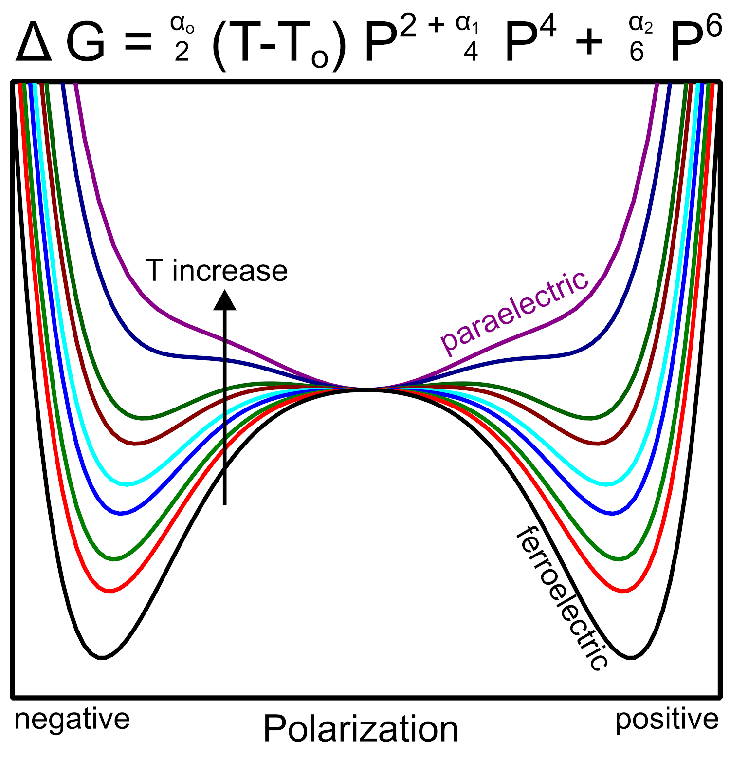
Free energy as a function of polarization and temperature, illustrative example showing how a material transitions from ferroelectric to paraelectric.
Spontaneous alignment (i.e. no external field) of neighboring unit cell dipole moments will eventually lead to the formation of domains which can have length scales beyond several nanometers. The formation of these domains is the typical criteria for classifying a material as being a ferroelectric The illustration below pictorially shows such phenomena,

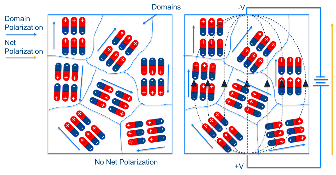
Example of domain polarization and external field induced net polarization (image adapted from https://ec.kemet.com/dielectric-polarization)

In the presence of an applied external electric field, the individual domains can will be driven to align with the field direction as to minimize the free energy, $ G = P_{i}E_{i}$. One can also write the difference in free energy, $\Delta G$, due to changes in the domain orientation such that:
\begin{align}
\Delta G &= G_{P_1} - G_{P_2} \\
&= \Delta P^s E_{i} + \frac{1}{2} \Delta \chi_{ij} E_i E_j
\end{align}
in the expressions above we use $i,j,\cdots$ tensor notation (a.k.a Einstein summation) to indicate coordinates. The term $P^s$ is the spontaneous polarization term and $\chi_{ij}$ susceptibility tensor.  The $\Delta$ in front of the material parameters indicates the difference in values between the two states. The change in free energy drives the domains so that they both align and spatial grow until a saturation condition is meet. The change in domain structure has lowered the configurational entropy and "poled" domain structure no longer remembers the initially random polarization configuration. This leads to a a hysteresis curve, where upon reversal of the applied electric field a different polarization configuration is sampled. I will have a blog on hysteresis phenomena.

The quote for today is an excerpt from one of the original documents highlighting the discovery of electric polarization and piezoelectric effects in a mineral salt (Rochelle salt):

"It appears then, that the asymmetry of the throws in Anderson's experiment is due to a hysteresis in electric polarization analogous to magnetic hysteresis. This would suggest a parallelism between the behavior of Rochelle salt as a dielectric and steel, for example, as a ferromagnetic substance."
- Joseph Valasek, APS Minutes, 1920

References & Additional Reading


Reuse and Attribution

Thursday, June 6, 2019

Ideal Solution Mixing: A-B Lattice


Here we will review the ideal solution mixing model for simple A-B lattice random mixing alloy system. The first step is to recall that for any system (e.g. state or phase) we can write the Gibbs free energy as:
$$ G = H-TS $$
where $H$ is the enthalpy, $T$ the temperature, and $S$ the entropy. We now propose that we have two isolated systems, lattice A and lattice B, and we want to find the change in Gibbs free energy when the two are combined to form a lattice with both A and B sites (randomly). An illustrative example would look something like below.


The next step is to write the change in Gibbs free energy as:
\begin{align}
\Delta G^{mix} & = G_{initial} - G_{final} \\
& = \Delta H^{mix} - T \Delta S^{mix} \\
\end{align}
Notice that we are using the label $mix$ to indicate that the change in Gibbs free energy is due to the mixing of the two lattices into one (i.e. Gibbs free energy of mixing).

In the ideal solution mixing model, we first approximate that $\Delta H^{mix}$  is negligible and taken to be zero. We can think of this as meaning that we assume no change in internal energy due to the chemical interactions between A and B. The next assumption is that the change in entropy is strictly due to configurational arrangement of A and B points on the combined lattice. This means that entropic effects due to lattice vibrations or magnetic ordering are not accounted for. Thus the Gibbs free energy has a simple relation to entropy:
$$ \Delta G^{mix} = - T \Delta S^{c} $$
The next step is to define the representation for the configurational entropy. To do this we will use to facts that each microstate is probabilistic and given by the combinatorics (i.e. possible configurations ). This is compactly represented by the famous equation:
$$ S^{c} = k_b \ln \omega^{c} $$
with $k_b$ being the Boltzmann constant and $\omega^{c}$ the configuration combinatorics. For the lattice AB this is going to be given by:
$$ \omega^{c} = \frac{N!}{N_{A}!N_{B}!}$$
where $N=N_{A}+N_{B}$ and $N_{A}$ and $N_{B}$ are the number of sites of a given type. At first glance calculating the configurational entropy may not seem daunting, however, logarithms of factorials can become demanding to calculate very quickly. Fortunately enough there is an approximation provided by mathematician James Stirling that allows one to approximate logarithms of factorials and is given by:
$$ \ln N! \approx N \ln N - N $$
Using this approximation we can determine $\omega^{c}$ and distill the expression of $S^{c}$ into something that is relative compact and meaningful. Apply the approximation we get:
\begin{align}
 \ln \omega^{c} &= N \ln N - N - \left[\ln\left(N_{A}!N_{B}!\right)\right] \\
&= N \ln N - N - \left[ N_{A} \ln N_{A} - N_{A} + N_{B} \ln N_{B} - N_{B}\right] \\
&= N \ln N - N_{A} \ln N_{A} - N_{B} \ln N_{B} - N + N_A + N_B \\
\end{align}
The last three terms cancel out, e.g., $N_A + N_B = N$ and we then rewrite the first term as:
\begin{align}
\ln \omega^{c} &= \left(N_A + N_B\right) \ln N  - N_{A}\ln N_A - N_{B}\ln N_B \\
&=-\left[N_A \ln \left(\frac{N_A}{N}\right) + N_{B}\ln\left( \frac{N_B}{N}\right) \right]
\end{align}
the ratio of $X_A = \frac{N_A}{N}$ or $X_B = \frac{N_B}{N}$  are the fraction of sites on the mixed lattice with A and B sites, respectively. Let us take one further step by multiplying the equation above by $\frac{N}{N}$ to get
$$ \ln \omega^{c} = -N \left[ X_A \ln X_A + X_B \ln X_B \right] $$
Now we can write $\Delta S^{mix}$ as,
$$ \Delta S^{mix} = -k_{b} N \left[ X_A \ln X_A + X_B \ln X_B \right] $$
if we assume that the total number of N sites on the alloy lattice is comparable to the number of particles in 1 mole, i.e., Avogadro's number $N_a = \text{6.022}\times \text{10}^{\text{23}}$, then we can write the Gibbs free energy of mixing in most familiar form as:
\begin{align}
 \Delta G^{mix} &= -T \Delta S^{mix} \\
&= -T \cdot -k_{b} N_{a} \left[ X_A \ln X_A + X_B \ln X_B \right]  \\
&= \boxed{RT \left[ X_A \ln X_A + X_B \ln X_B \right]}
\end{align}
where $R$ is the gas constant given by  $k_b N_a$. We can get a sense for how the Gibbs free energy of mixing changes with temperature as shown in the graph below,


From the graph we observe two features, 1.) the Gibbs free energy of mixing for an ideal solution is a symmetric function, 2.) as the temperature is increased $\Delta G^{mix} is decreases. Not that in the graph the line(s) do not extend to zero and one, this is because these would be given by the Gibbs free energy of the reference states of lattice A and B.

Ideal solution mixing is typically not suitable for real material alloy systems and thus other approximations such as the regular solution model are used. In the regular solution model we use the same $\Delta S^{mix}$ and include a non-zero expression for $\Delta H^{mix}$. The most accurate approach for calculating Gibbs free energy of mixing for real materials is to use CALPHAD methodologies.

For this blog postings quote we will get two quotes:

"Nothing in life is certain except death, taxes and the second law of thermodynamics."
-Seth Lloyd, MIT Professor 

"In this house, we obey the laws of thermodynamics!"
-Homer Simpson, response to Lisa's perpetual motion machine

References & Additional Reading

Reuse and Attribution